Popular Activation Functions & Implementation

I go by theroyakash on the internet. I am a computer scientist, with research in high performance algorithms, data structures, distributed systems, and beyond. See my work searching google for theroyakash.
Here in this post we'll be implementing popular deep learning activation functions from the ground up using numpy.
So for you to follow this post you need to things:
numpyand- Some free time of yours.
If you have written any deep learning code before you likely have used these activations:
- Softmax
- ReLU, LeakyReLU
- and the good-old Sigmoid activation.
In this post I'll implement all these activation functions with numpy and also the derivative of these for the back-propagation.
ReLU
Let's get the easy one out first. ReLU is called rectified linear unit, where:

class ReLU:
    """Applies the rectified linear unit function element-wise.
        ReLU operation is defined as the following
    """

    def __call__(self, x):
        return np.where(x >= 0, x, 0)

    def gradient(self, x):
        """
        Computes Gradient of ReLU
            Args:
                x: input tensor
            Returns:
                Gradient of X
        """
        return np.where(x >= 0, 1, 0)
Usage:
relu = ReLU()
z = np.array([0.1, -0.4, 0.7, 1])
print(relu(z))      # ---> array([0.1, 0. , 0.7, 1. ])
print(relu.gradient(z))   # ---> array([1, 0, 1, 1])
Sigmoid
Sigmoid function is defined as the following

The main reason why we use sigmoid function is because it exists between (0 to 1). Therefore, it is especially used for models where we have to predict the probability as an output.Since probability of anything exists only between the range of 0 and 1, sigmoid is the right choice. The function is differentiable.That means, we can find the slope of the sigmoid curve at any two points. The function is monotonic but function’s derivative is not. The logistic sigmoid function can cause a neural network to get stuck at the training time. The softmax function is a more generalized logistic activation function which is used for multi-class classification.
The element wise exp can be done like the following, and if you calculate the derivative you can find that d/dx sigmoid(x) = sigmoid(x) *(1- sigmoid(x)).

So let's write up the activation function for sigmoid operation:
class Sigmoid:
    """
    Applies the element-wise function
    Shape:
        - Input: :math:`(N, *)` where `*` means, any number of additional
          dimensions
        - Output: :math:`(N, *)`, same shape as the input
    """

    def __call__(self, x):
        return 1 / (1 + np.exp(-x))

    def gradient(self, x):
        r"""Computes Gradient of Sigmoid
        .. math::
            \frac{\partial}{\partial x} \sigma(x) = \sigma(x)* \left (  1- \sigma(x)\right)
        Args:
            x: input tensor
        Returns:
            Gradient of X
        """

        return self.__call__(x) * (1 - self.__call__(x))
and the usage would be like this:
import numpy as np

z = np.array([0.1, 0.4, 0.7, 1])
sigmoid = Sigmoid()
return_data = sigmoid(z)

print(return_data)          # -> array([0.52497919, 0.59868766, 0.66818777, 0.73105858])
print(sigmoid.gradient(z))  # -> array([0.24937604, 0.24026075, 0.22171287, 0.19661193])
LeakyReLU
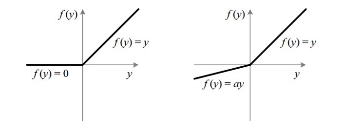
LeakyReLU operation is similar to the ReLU operation also called the Leaky version of a Rectified Linear Unit. It essentially instead of putting zeros everywhere it sees < 0, it puts an predefined -ve slope like -0.1 or -0.2 etc. You mention an alpha, and it'll put -alpha where X < 0.
The following image shows the difference between ReLU and LeakyReLU

class LeakyReLU:
    """Applies the element-wise function:
    Args:
        - alpha: Negative slope value: controls the angle of the negative slope in the :math:`-x` direction. Default: ``1e-2``
    """
    def __init__(self, alpha=0.2):
        self.alpha = alpha

    def __call__(self, x):
        return np.where(x >= 0, x, self.alpha * x)

    def gradient(self, x):
        """
        Computes Gradient of LeakyReLU
            Args:
                x: input tensor
            Returns:
                Gradient of X
        """
        return np.where(x >= 0, 1, self.alpha)
tanH or hyperbolic tangent activation
The sigmoid maps the output between 0-1 but here tanH maps the output to -1 and 1. The advantage is that the negative inputs will be mapped strongly negative and the zero inputs will be mapped near zero in the tanh graph.
The function is differentiable. And the function is monotonic while its derivative is not monotonic. The tanH function is mainly used classification between two classes.
Let's implement this in code
class TanH:
    def __call__(self, x):
        return 2 / (1 + np.exp(-2 * x)) - 1

    def gradient(self, x):
        return 1 - np.power(self.__call__(x), 2)
Softmax
Softmax loss is used when multi-class classifications are performed. So here is the code:
class Softmax:
    def __call__(self, x):
        e_x = np.exp(x - np.max(x, axis=-1, keepdims=True))
        return e_x / np.sum(e_x, axis=-1, keepdims=True)

    def gradient(self, x):
        p = self.__call__(x)
        return p * (1 - p)


![Set-up an audio version of your blog articles [Works Automatically]](/_next/image?url=https%3A%2F%2Fcdn.hashnode.com%2Fres%2Fhashnode%2Fimage%2Fupload%2Fv1612940767582%2F0abS3UT_8.png&w=3840&q=75)

